Analytical DFG Term for IBL

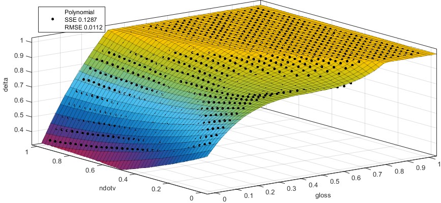
Image-based lighting is an important part of a physically based rendering. Unfortunately straightforward IBL implementation for more complicated lighting models than Phong requires a huge lookup table and isn’t practical for real time. Current state of the art approach is split sum approximation [Kar13], which decomposes IBL integral into two terms: LD and DFG. LD is stored in standard cube map and DFG is stored in one global 2D LUT texture. This texture is usually 128×128 R16G16F, contains scale and bias for specular color and is indexed by roughness/gloss and ndotv. DFG LUT is quite regular and looks like it could be efficiently approximated by some kind of low order polynomial.

My main motivation was to create a custom 3ds Max shader, so artists could see how their work will look in our engine. Of course 3ds Max supports custom textures, but it’s not very user friendly and error prone when artists need to assign some strange LUT texture. It’s better to hide such internal details. Furthermore it can be beneficial for performance, as you can replace memory lookup with ALU. Especially on bandwidth constrained platforms like mobile devices.

Surface fitting

There are many surface fitting tools, which given some data points and equation, automatically find best coefficients. It’s also possible to transform curve fitting problem into a nonlinear optimization problem and use tool designed for solving them. I prefer to work with Matlab, so of course I used Matlab’s cftool. It’s a separate application with GUI. You just enter an equation and it automatically fits functions, plots surface against data points and computes error metrics like SSE or RMSE. Furthermore you can compare side by side with previous approximations. Popular Mathematica can also easily fit surfaces (FindFit), but it requires more work, as you need to write some code for plotting and calculating error metrics.

Usually curve fitting is used for smoothing data, so most literature and tools focus on linear functions like polynomial and Gaussian curves. For real-time rendering polynomial curves are most cost efficient on modern scalar architectures like GCN. Polynomial curves avoid costly transcendentals (exp2, log2 etc.), which are quarter rate on GCN. For extra quality add freebies like saturate or abs to constrain function output. In some specific cases it’s worth to add other full rate instructions like min, max or cndmask.

Most fitting is done with non linear functions, where fitting tools often are stuck in a local solution. In order to find a global one you can either write a script which fits for different starting points and compares results or just try a few points by hand until plotted function will look good. For more complicated cases there are smarter tools for finding global minimum like Matlab’s MultiStart or GlobalSearch.

Last thing is not only to try polynomial of some order, but also play with all it’s variables. Usually I first search for order of polynomial which properly approximates given data and then try to remove higher order variables and compare results. This step could be automatized to check all variable combinations. I never did it, as higher order are impractical for real time rendering, so there aren’t too many combinations.

DFG LUT

First I tried to generate LUT inside Matlab, but it was too slow compute, so I switched to C++ and loaded that LUT as CSV. Full C++ source for LUT generation is on Github. It uses popular GGX distribution, Smith geometry term and Schlick’s Fresnel approximation. Additionally I use roughness remap  which results results in similar distribution to Blinn-Phong . This remap is also similar to , which was used by Crytek in Ryse [Sch14].

for ( unsigned y = 0; y < LUT_HEIGHT; ++y )
{
float const ndotv = ( y + 0.5f ) / LUT_WIDTH;

for ( unsigned x = 0; x < LUT_WIDTH; ++x )
{
float const gloss = ( x + 0.5f ) / LUT_HEIGHT;
float const roughness = powf( 1.0f - gloss, 4.0f );

float const vx = sqrtf( 1.0f - ndotv * ndotv );
float const vy = 0.0f;
float const vz = ndotv;

float scale = 0.0f;
float bias = 0.0f;

for ( unsigned i = 0; i < sampleNum; ++i )
{
float const e1 = (float) i / sampleNum;
float const e2 = (float) ( (double) ReverseBits( i ) / (double) 0x100000000LL );

float const phi = 2.0f * MATH_PI * e1;
float const cosPhi = cosf( phi );
float const sinPhi = sinf( phi );
float const cosTheta = sqrtf( ( 1.0f - e2 ) / ( 1.0f + ( roughness * roughness - 1.0f ) * e2 ) );
float const sinTheta = sqrtf( 1.0f - cosTheta * cosTheta );

float const hx = sinTheta * cosf( phi );
float const hy = sinTheta * sinf( phi );
float const hz = cosTheta;

float const vdh = vx * hx + vy * hy + vz * hz;
float const lx = 2.0f * vdh * hx - vx;
float const ly = 2.0f * vdh * hy - vy;
float const lz = 2.0f * vdh * hz - vz;

float const ndotl = std::max( lz, 0.0f );
float const ndoth = std::max( hz, 0.0f );
float const vdoth = std::max( vdh, 0.0f );

if ( ndotl > 0.0f )
{
float const gsmith = GSmith( roughness, ndotv, ndotl );
float const ndotlVisPDF = ndotl * gsmith * ( 4.0f * vdoth / ndoth );
float const fc = powf( 1.0f - vdoth, 5.0f );

scale += ndotlVisPDF * ( 1.0f - fc );
bias += ndotlVisPDF * fc;
}

scale /= sampleNum;
bias /= sampleNum;
}
}
}

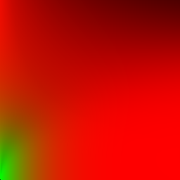
Code above outputs texture like this:

Approximation

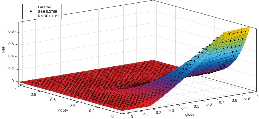
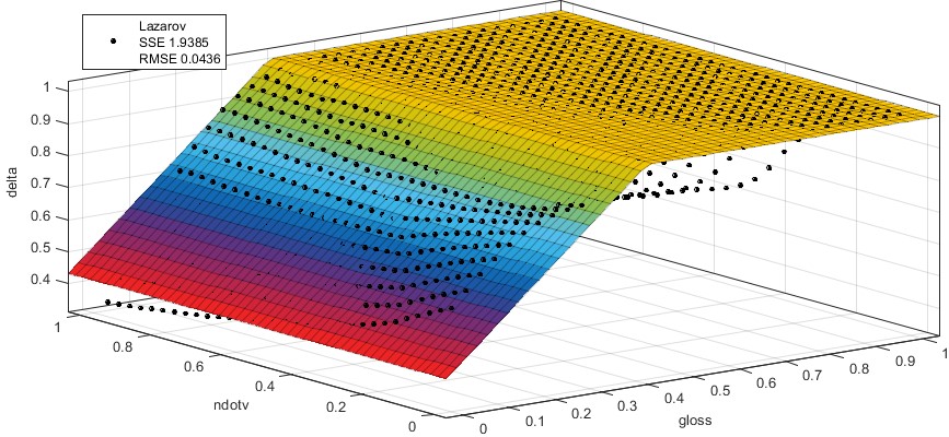
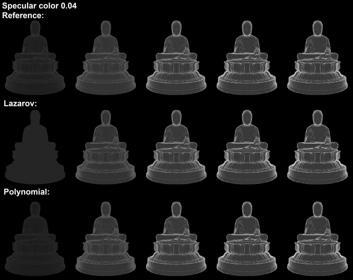
[Laz13] presented an analytical solution to DFG term. He used Blinn-Phong distribution, so first I fitted his approximation for GGX and my roughness remap. Instead of storing scale directly, delta is used (scale = delta – bias). It simplifies fitting as delta is a simpler surface than scale. Additionally to get a tighter fit I added saturate for bias and delta values.

float3 EnvDFGLazarov( float3 specularColor, float gloss, float ndotv )
{
float4 p0 = float4( 0.5745, 1.548, -0.02397, 1.301 );
float4 p1 = float4( 0.5753, -0.2511, -0.02066, 0.4755 );

float4 t = gloss * p0 + p1;

float bias = saturate( t.x * min( t.y, exp2( -7.672 * ndotv ) ) + t.z );
float delta = saturate( t.w );
float scale = delta - bias;

bias *= saturate( 50.0 * specularColor.y );
return specularColor * scale + bias;
}

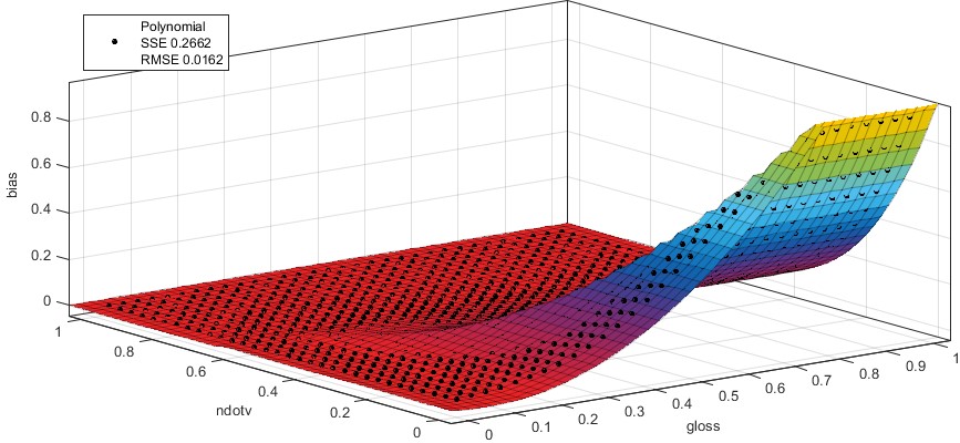
Then I tried to find a better approximation. I focused on simple instructions in order to avoid transcendentals like exp, which are quarter rate on GCN. I tried many ideas for bias fitting – from simple polynomials to expensive Gaussians. Finally settled on two polynomials oriented to axes and combined with min. One depends only on x and second only on y. Fitting delta was easy – 2nd order polynomial with some additional term did the job.

float3 EnvDFGPolynomial( float3 specularColor, float gloss, float ndotv )
{
float x = gloss;
float y = ndotv;

float b1 = -0.1688;
float b2 = 1.895;
float b3 = 0.9903;
float b4 = -4.853;
float b5 = 8.404;
float b6 = -5.069;
float bias = saturate( min( b1 * x + b2 * x * x, b3 + b4 * y + b5 * y * y + b6 * y * y * y ) );

float d0 = 0.6045;
float d1 = 1.699;
float d2 = -0.5228;
float d3 = -3.603;
float d4 = 1.404;
float d5 = 0.1939;
float d6 = 2.661;
float delta = saturate( d0 + d1 * x + d2 * y + d3 * x * x + d4 * x * y + d5 * y * y + d6 * x * x * x );
float scale = delta - bias;

bias *= saturate( 50.0 * specularColor.y );
return specularColor * scale + bias;
}

Some screenshots comparing reference and two approximations:

Instruction histograms on GCN architecture:

	Lazarov	Polynomial fit
v_exp_f32	1
v_mac_f32	3	3
v_min_f32	1	1
v_mov_b32	4	2
v_mul_f32	1	5
v_add_f32		2
v_madmk_f32		4
v_mad_f32	2	1
v_subrev_f32	1	1
total cycles:	16	19

Conclusion

To sum up I presented here a simple analytical function for DFG approximation. In practice it’s hard to distinguish this approximation from reference and it uses a moderate amount of ALU.

References

[Kar13] B. Karis – “Real Shading in Unreal Engine 4”, Siggraph 2013
[Laz13] D. Lazarov – “Getting More Physical in Call of Duty: Black Ops II”, Siggraph 2013
[Sch14] N. Schulz – “The Rendering Technology of Ryse”, GDC 2014